Workload Evaluation

2026-03-07 19:28

Workload Evaluation

There are generally three main factors that affect computer systems' performance:

The design of the system
Implementation of the system
Workload to which the system is subjected

Possibly the worst thing about evaluating workload is summarized in the GIGO principal (garbage-in-garbage-out). Using the wrong metrics and signals can lead to irrelevant noisy results that cannot be relied on.

Importance of Workloads

Complete system evaluations are often modeled like an algorithm in the sense that they can work very well in one scenario but not all.

Consider the following examples:

Example 1: Scheduling parallel jobs by size

The simple intuitive way to solve this problem is by modeling it in the form of resources x time. Every process will need a certain amount of processors within a certain interval of time. This creates a bunch of small rectangles that we have to then arrange them into a larger rectangle that represents all the available resources.

One famous problem shows up here with the SJF algorithm (Short Job First); that is, our short process will starve the other procs of resources if it keeps requesting to run (which we cannot predict since that will happen at runtime). In parallel systems, scheduling things based on size can also have the side effect of scheduling by duration.

One must not however assume such correlation. We have instead created some models to predict said relation:

Fixed Work: This assumes that the job will be doing a known set of instructions and parallelism is merely solved to solve the same problem but faster. This is generally the case with a lot of simple GPU programming applications. This means that there is a negative correlation between the runtime and the degree of parallelism in ths case.
Fixed Time: In this case we use parallelism to solve something else under the assumption that runtime stays fixed. Thus, runtime would not be correlated with the degree of parallelism.
Memory Bound: If the problem size is increased to fill the memory associated with processors, the amount of productive work typically grows at least linearly with the parallelism. The overheads associated with parallelism always grow super-linearly. Thus the runtime is positively correlated with parallelism.

This is just to show that different systems can utilize the model of scheduling based on the number of processors used. For an uncorrelated or negatively correlated workload, it is fine to use this scheme. However, a positively correlated workload will mean that procs with more processors will dominate the runtime and starve the smaller procs from resources.

After enumerating the models that might reflect the workload in question, one must ask which of those models is realistic; in this case for example, we don't actually expect to have a fixed-work workload so the other two are more related. This will mean that choosing the scheduling algorithm outlined above is probably a bad idea since it, at best, does not favor smaller jobs which will probably increase the average response time.

Example 2: Processor allocation using a buddy system

Another way to schedule things could be using time-slicing with coordinated context switching on all processors. So the processes of one job are scheduled on all processors (given all resources) and then we switch them with other procs from another job. This is known as Gang scheduling and we normally use something called Ousterhout matrix where columns are processors and rows are time slots. How do we include the job information in said matrix you ask?

DHC Schemes could be used to create a buddy system for each processor allocation:

Divide resources into a power of 2
Round up each request to the next power of 2 (if a job requests 5 processors, give it 8)
This gives us the ability to reuse the same block permutation in future time slots
1. i.e., proc A can reuse 0-7 if those become free in the future..

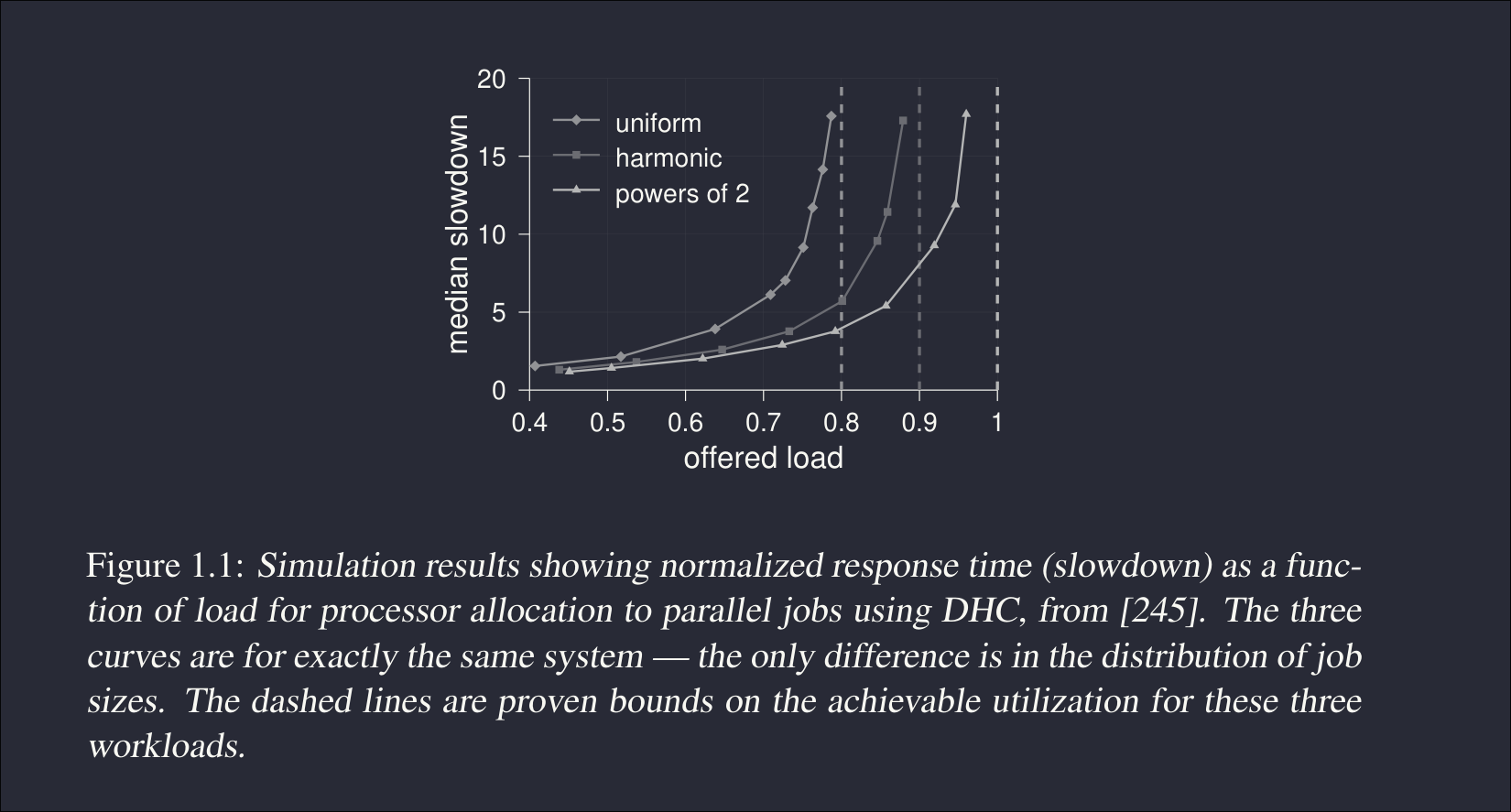
Looking at the figure above, we can see that a uniform distribution of job sizes (all sizes are equally likely) can lead to major slowdowns at normal reasonably high load. This should be trivial because a bunch of jobs that are not a power of 2 will be extremely annoying to deal with as we round up resources. Harmonics are a bit better since we are more likely to get smaller requests so even if we round these up, it will not starve the system much.

Example 3: Load balancing on a Unix cluster

This is a way of having equity among servers. Just move jobs from overloaded machines to a more free one :)
One common problem here is which process to migrate from sad machine.. There are few things to keep in mind here:

There is a significant amount of overhead in this migration.
If a process terminates shortly after migration, then it was a waste.
The process needs to be suspended while migrating.

Selecting which process is likely to continue running is slightly subtle. We obviously should not select a job at random because most jobs tend to be short realistically. The best indication that a process will continue to run after migration is if it was running for a while already. In other words, we can use the fact that the process took long to consider it a tea-drinking buddy.

Quote

Runtime Distributions and What They Tell Us About the Future

Let $T$ denote the runtime of a process. A scheduler would like to estimate how much longer a process will run given that it has already run for time $t$ .

Exponential runtimes (memoryless case).

If runtimes follow an exponential distribution, then

P r (T > t + τ ∣ T > t) = P r (T > τ)

This means that the past contains no information about the future. A process that has already run for a long time is statistically identical to a newly started one. Consequently, the expected remaining runtime is always equal to the mean of the distribution, regardless of how long the process has already run.

Intuition: the system behaves like repeated coin flips — the past does not influence the future.

Real workloads (heavy-tailed runtimes).

Empirical studies of Unix workloads show that runtimes are not exponential but heavy-tailed:

P r (T > τ) \propto τ^{- α}, α \approx 1

This implies:

Most processes are short.
A small fraction are extremely long.

Under such distributions, conditioning on elapsed runtime changes the expectation:
if a process has already run for time $t$ , its expected remaining runtime is roughly proportional to $t$ .

Intuition: long-running processes reveal themselves by simply surviving long enough.

Scheduling implication.

Because of heavy tails:

Randomly selecting a process will most likely pick a short job.
Selecting processes that have already run the longest preferentially identifies the true long-running jobs.

Therefore, runtime observed so far becomes a useful signal for decisions such as migration or load balancing.

TLDR.

The usefulness of runtime as a predictor depends entirely on the statistical structure of the workload.
It is useless under memoryless (exponential) assumptions, but highly informative under the heavy-tailed distributions observed in real systems.

References

Scheduling (computing)
Amdahl's law

Tags:

Software
Statistics