Poisson Distribution

2025-07-21 09:07

Tags: #mathematics #engineering #probability

Poisson Distribution

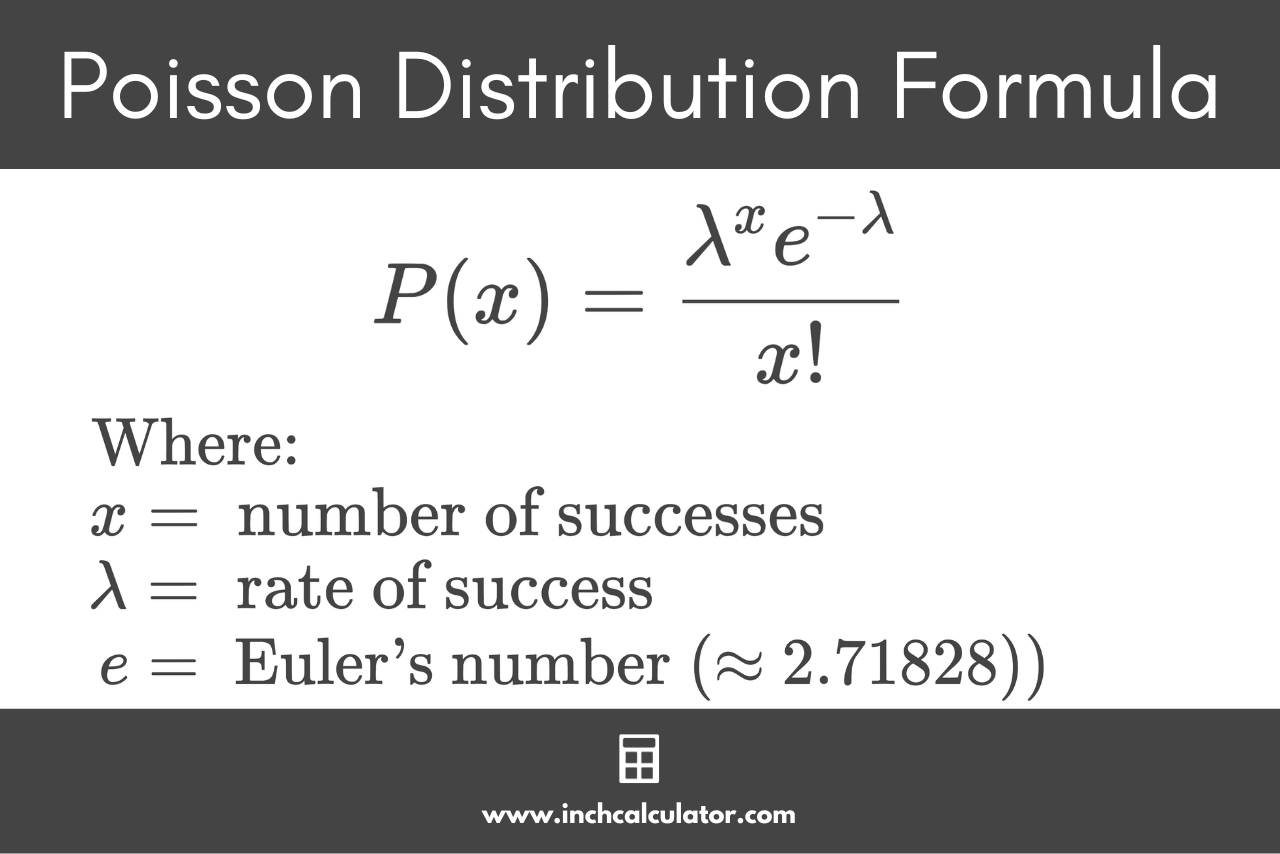
The Poisson distribution typically models the number of events occurring in a fixed interval of time or space, given that:

The events occur independently of each other.
The average rate of occurrence (denoted by 𝜆) is constant throughout the interval.
The probability of more than one event happening in an infinitesimally small interval is negligible.

Consider a fixed time interval, say from 0 to T, and let the number of events that occur in this interval be k. The number of events is modeled by a random variable X.

Let the rate of occurrence of events be 𝜆, meaning the expected number of events in the interval T is 𝜆T.
We divide the interval T into n smaller sub-intervals of length delta(t) = T/n, where n is large and delta t is small.

For each sub-interval, we assume the following:

The probability of exactly one event occurring in the sub-interval is proportional to delta t
The probability of more than one event occurring in the sub-interval is negligible because delta t is small
The number of events in each sub-interval is independent of others.

Thus, the probability P(one event in a sub-interval) is proportional to 𝜆Δt
Probability of no event occurring is 1-𝜆Δt

Now, for the entire interval T, the number of events X must follow a binomial distribution, where:

We have n trials (each sub-interval)
The probability of success (an event happening) in each trial is p1 = 𝜆Δt
The total number of events k is the sum of successes in these n trials.

The binomial probability mass function (PMF) for observing k events is given by:

P (X = k) = (\binom{n}{k}) (λ Δ t)^{k} (1 - λ Δ t)^{n - k}

This essentially gives the probability of getting k successes/events out of n trials.

As n goes to infinity, we will have smaller time intervals. And we know that nΔt is T which is a fixed constant.

Under this limit, the binomial turns into the Poisson distribution!

Key Approximations

As n approaches infinity, and as the interval gets smaller we can say that

lim_{n \to \infty} (1 - \frac{x}{n}) = e^{- x}

For large n and fixed k, we approximate:

(\binom{n}{k}) (λ Δ t)^{k} \approx \frac{(n λ Δ t)^{k}}{k!} = \frac{(λ T)^{k}}{k!}

References

Binomial distribution

Tags:

Mathematics
Engineering
Probability